Predicting the winner
Firstly we need to import some modules to help us along the way.
1
2
3
4
5
6
7
| import matplotlib.pyplot as plt
import pandas as pd
import numpy as np
from scipy.stats import poisson, skellam
import matplotlib.mlab as mlab
import math
from collections import Counter
|
Then we want to read the data file into our program.
1
| data = pd.read_csv("resources/PremierLeague1718.csv") # Read the data set file
|
The data file consists of empty columns and rows which we want to clean up so that we are working with clean data. To do this we can use the below function.
1
2
3
| def clean(dataframe):
assert isinstance(dataframe, pd.DataFrame), 'Argument of wrong type!'
return dataframe.dropna(axis=1, how='all')
|
And then we can apply this to our data.
1
| data = clean(data) # Clean the data up to remove empty and NaN cols
|
Because the data file consists of a lot of columns, some of them are irrelevant to us, the below function can help eliminate these columns, to do this we can specify only the columns we want to keep as a list of column names.
1
2
3
4
| def filterCols(dataframe, cols):
assert isinstance(dataframe, pd.DataFrame), 'Argument of wrong type!'
assert isinstance(cols, list), 'Argument of wrong type!'
return dataframe[cols]
|
We can then use this function to filter our data.
1
2
| colsToKeep = ["Date", "HomeTeam", "AwayTeam", "FTHG", "FTAG", "HS", "AS", "HST", "AST", "FTR"] # List of cols we want to keep
data = filterCols(data, colsToKeep) # Filter relevant cols
|
To get an idea of how the data looks like, we can use the describe function to give us various information. (This is helpful to answer Question 1, part 1.)
1
2
| print("Description:")
print(data.describe())
|
1
2
3
4
5
6
7
8
9
10
| Description:
FTHG FTAG HS AS HST AST
count 240.000000 240.000000 240.000000 240.000000 240.000000 240.000000
mean 1.491667 1.183333 13.666667 11.141667 4.554167 3.791667
std 1.344419 1.250830 6.055301 5.110160 2.781661 2.385086
min 0.000000 0.000000 2.000000 1.000000 0.000000 0.000000
25% 0.000000 0.000000 9.000000 7.000000 2.750000 2.000000
50% 1.000000 1.000000 13.000000 10.000000 4.000000 3.500000
75% 2.000000 2.000000 17.000000 14.000000 6.000000 5.000000
max 7.000000 6.000000 35.000000 30.000000 15.000000 14.000000
|
Furthermore, we can also group the data in a way so that we can see an outlook of how many goals were scored and conceded by each team over the whole league.
1
2
3
4
5
6
7
8
9
10
11
12
13
14
15
16
17
18
19
20
| def renameCols(df, colsdict):
return df.reset_index().rename(columns=colsdict)
def creategroups():
groups = [0,0,0,0]
groups[0] = renameCols(data.groupby("HomeTeam")["FTR"].apply(lambda x: x[x == 'H'].count()), {"HomeTeam": "Team", "FTR": "Wins at home"})
groups[1] = renameCols(data.groupby("AwayTeam")["FTR"].apply(lambda x: x[x == 'A'].count()), {"AwayTeam": "Team", "FTR": "Wins away"})
groups[2] = renameCols(data.groupby("HomeTeam")["FTR"].apply(lambda x: x[x == 'A'].count()), {"HomeTeam": "Team", "FTR": "Losses at home"})
groups[3] = renameCols(data.groupby("AwayTeam")["FTR"].apply(lambda x: x[x == 'H'].count()), {"AwayTeam": "Team", "FTR": "Losses away"})
return groups
groups = creategroups()
merged = groups[0].merge(groups[1], on="Team").merge(groups[2], on="Team").merge(groups[3], on="Team")
print("Data on wins/losses")
print(merged)
print("Averages of the wins/losses")
print(merged.describe())
|
1
2
3
4
5
6
7
8
9
10
11
12
13
14
15
16
17
18
19
20
21
22
23
24
25
26
27
28
29
30
31
32
| Data on wins/losses
Team Wins at home Wins away Losses at home Losses away
0 Arsenal 9 3 1 5
1 Bournemouth 4 2 5 6
2 Brighton 3 2 3 8
3 Burnley 5 4 5 3
4 Chelsea 8 7 2 2
5 Crystal Palace 4 2 4 7
6 Everton 6 1 4 6
7 Huddersfield 4 2 4 8
8 Leicester 6 3 4 4
9 Liverpool 7 6 0 3
10 Man City 11 10 0 1
11 Man United 9 7 1 2
12 Newcastle 3 3 6 7
13 Southampton 3 1 5 5
14 Stoke 5 1 5 8
15 Swansea 3 2 7 7
16 Tottenham 7 6 1 4
17 Watford 3 4 5 7
18 West Brom 2 1 3 7
19 West Ham 4 2 4 6
Averages of the wins/losses
Wins at home Wins away Losses at home Losses away
count 20.000000 20.000000 20.000000 20.000000
mean 5.300000 3.450000 3.450000 5.300000
std 2.494204 2.502104 2.012461 2.202869
min 2.000000 1.000000 0.000000 1.000000
25% 3.000000 2.000000 1.750000 3.750000
50% 4.500000 2.500000 4.000000 6.000000
75% 7.000000 4.500000 5.000000 7.000000
max 11.000000 10.000000 7.000000 8.000000
|
We can create a data structure containing information about the teams we care about. In this instance Manchester United and Manchester City. This can help us answer Question 1 part 2.
1
2
3
4
5
6
7
8
9
10
11
12
13
14
15
16
17
18
19
20
21
22
23
| rteams = ["Man United", "Man City"] # Teams we care about
teams = {"ManUnitedHome": "", "ManCityHome": "", "ManUnitedAway": "", "ManCityAway": ""} # A dict to contain relevant team dataframes
teams["ManUnitedHome"] = data.loc[data["HomeTeam"] == "Man United"]
teams["ManUnitedAway"] = data.loc[data["AwayTeam"] == "Man United"]
teams["ManCityHome"] = data.loc[data["HomeTeam"] == "Man City"]
teams["ManCityAway"] = data.loc[data["AwayTeam"] == "Man City"]
def mergeteamdata():
df = teams["ManUnitedHome"].append(teams["ManUnitedAway"])
df = df.append((teams["ManCityHome"].append(teams["ManCityAway"])))
return df
print("Man United Home:")
print(teams["ManUnitedHome"].describe())
print("\nMan City Home")
print(teams["ManCityHome"].describe())
print("-------------")
print("Man United Away:")
print(teams["ManUnitedAway"].describe())
print("\nMan City Away")
print(teams["ManCityAway"].describe())
|
1
2
3
4
5
6
7
8
9
10
11
12
13
14
15
16
17
18
19
20
21
22
23
24
25
26
27
28
29
30
31
32
33
34
35
36
37
38
39
40
41
42
43
| Man United Home:
FTHG FTAG HS AS HST AST
count 12.000000 12.000000 12.000000 12.000000 12.000000 12.000000
mean 2.250000 0.416667 16.250000 9.666667 5.500000 3.666667
std 1.484771 0.792961 5.047502 3.420083 2.110579 2.059715
min 0.000000 0.000000 8.000000 3.000000 2.000000 1.000000
25% 1.000000 0.000000 14.000000 7.750000 3.750000 2.000000
50% 2.000000 0.000000 16.000000 10.000000 6.000000 3.500000
75% 4.000000 0.250000 20.500000 12.250000 7.000000 5.000000
max 4.000000 2.000000 23.000000 14.000000 9.000000 7.000000
Man City Home
FTHG FTAG HS AS HST AST
count 12.000000 12.000000 12.000000 12.000000 12.000000 12.000000
mean 3.500000 0.750000 18.583333 6.500000 8.333333 2.166667
std 1.623688 0.621582 5.177896 1.381699 2.386833 1.466804
min 1.000000 0.000000 9.000000 5.000000 5.000000 0.000000
25% 2.750000 0.000000 14.750000 5.750000 6.750000 1.000000
50% 3.000000 1.000000 19.500000 6.500000 8.500000 2.000000
75% 4.250000 1.000000 21.750000 7.000000 10.250000 3.250000
max 7.000000 2.000000 26.000000 10.000000 12.000000 4.000000
-------------
Man United Away:
FTHG FTAG HS AS HST AST
count 12.000000 12.000000 12.00000 12.000000 12.000000 12.000000
mean 0.916667 1.833333 13.75000 12.666667 4.500000 4.500000
std 0.900337 1.337116 7.28791 5.087120 3.919647 2.430862
min 0.000000 0.000000 5.00000 6.000000 0.000000 1.000000
25% 0.000000 1.000000 10.75000 8.750000 2.750000 2.750000
50% 1.000000 2.000000 12.00000 11.000000 3.500000 4.000000
75% 2.000000 2.250000 15.00000 17.250000 5.000000 6.250000
max 2.000000 4.000000 33.00000 21.000000 15.000000 8.000000
Man City Away
FTHG FTAG HS AS HST AST
count 12.000000 12.000000 12.000000 12.000000 12.000000 12.000000
mean 0.750000 2.333333 7.083333 17.000000 2.500000 6.083333
std 1.215431 1.556998 3.579191 5.063236 2.067058 2.234373
min 0.000000 0.000000 2.000000 11.000000 0.000000 4.000000
25% 0.000000 1.750000 5.500000 14.000000 1.000000 4.000000
50% 0.000000 2.000000 6.500000 15.000000 2.000000 5.500000
75% 1.000000 3.000000 8.250000 19.750000 3.250000 7.250000
max 4.000000 6.000000 16.000000 28.000000 7.000000 10.000000
|
To get a better visualisation of how these teams stack up against eachother we can plot these values onto a graph t compare Manchester United’s home defence against Manchester City’s away offence and Manchester City’s home defence against Manchester United’s away offence.
1
2
3
4
5
6
7
8
9
10
11
12
13
14
15
16
| def plotstats(stat):
fig = plt.figure(1)
fig.set_size_inches(12, 8)
for i in stat:
plt.subplot(i.plots[0])
i.df.boxplot(i.col, vert=False)
plt.subplot(i.plots[1])
temp = i.df[i.col].as_matrix()
plt.hist(temp, bins=20, alpha=1, label=i.glabel)
plt.xlabel(i.xlabel)
plt.ylabel(i.ylabel)
plt.legend()
plt.xticks(np.arange(min(temp), max(temp)+1, 1.0))
plt.yticks(np.arange(0, len(temp)+1, 1.0))
plt.show()
|
We can create a simple object to use with the above function because it gives us a dynamic way of displaying information for different teams.
1
2
3
4
5
6
7
8
| class PlotObject:
def __init__(self, df, col, glabel, xlabel, ylabel, plots):
self.df = df
self.col = col
self.glabel = glabel
self.xlabel = xlabel
self.ylabel = ylabel
self.plots = plots
|
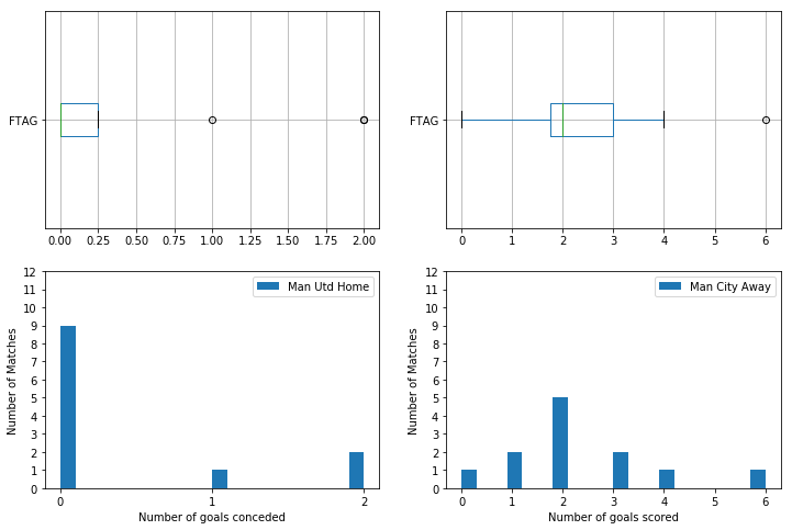
We can then plot these teams and see how the data looks like. This will help answer Question 1 part 3.
Manchester United’s home defence vs Manchester City’s away offence
1
2
3
4
| obj = []
obj.append(PlotObject(teams["ManUnitedHome"], "FTAG", "Man Utd Home", "Number of goals conceded", "Number of Matches", [221,223]))
obj.append(PlotObject(teams["ManCityAway"], "FTAG", "Man City Away", "Number of goals scored", "Number of Matches", [222,224]))
plotstats(obj)
|
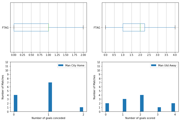
Manchester City’s home defence vs Manchester United’s away offence
1
2
3
4
| obj = []
obj.append(PlotObject(teams["ManCityHome"], "FTAG", "Man City Home", "Number of goals conceded", "Number of Matches", [221, 223]))
obj.append(PlotObject(teams["ManUnitedAway"], "FTAG", "Man Utd Away", "Number of goals scored", "Number of Matches", [222, 224]))
plotstats(obj)
|
Simulation
To simulate the future matches, we can use the poisson distribution to randomly generate future scores and see how the teams stack up against eachother.
1
2
3
| def sim_poisson(nums, mean):
gen = np.random.poisson(lam = mean, size = nums)
return gen
|
And then we can use this function to generate some scores for the following cases: Man Utd Home vs Man City Away Man City Home vs Man Utd Away
1
2
3
4
5
6
7
8
9
10
11
| def generate_scores():
gen_scores = []
gen_scores.append(sim_poisson(1000, teams["ManUnitedHome"]["FTHG"].mean()))
gen_scores.append(sim_poisson(1000, teams["ManUnitedAway"]["FTAG"].mean()))
gen_scores.append(sim_poisson(1000, teams["ManCityHome"]["FTHG"].mean()))
gen_scores.append(sim_poisson(1000, teams["ManCityAway"]["FTAG"].mean()))
MUHVSMCA = list(map(list,zip(gen_scores[0],gen_scores[3])))
MCHVSMUA = list(map(list,zip(gen_scores[2],gen_scores[1])))
return {"ManUtdHvsMC": MUHVSMCA, "ManCityHvsMU": MCHVSMUA}
|
1
| genscores = generate_scores()
|
We can summarise this data by looking at who won each game.
1
2
3
4
5
6
7
| def getresult(arr):
if arr[0] > arr[1]:
return "H"
elif arr[0] < arr[1]:
return "A"
else:
return "D"
|
1
| ManUtdHvsMC = [getresult(i) for i in (genscores["ManUtdHvsMC"])]
|
1
| ManCityHvsMU = [getresult(i) for i in (genscores["ManCityHvsMU"])]
|
1
2
3
4
| home_stats = {
"MU Win": Counter(ManUtdHvsMC)["H"],
"MC Win": Counter(ManCityHvsMU)["H"],
}
|
1
2
3
4
| away_stats = {
"MU Win": Counter(ManCityHvsMU)["A"],
"MC Win": Counter(ManUtdHvsMC)["A"],
}
|
1
| draws = Counter(ManCityHvsMU)["D"] + Counter(ManUtdHvsMC)["D"]
|
1
2
3
4
5
| df = pd.DataFrame(home_stats, index=["Home"])
df = df.append(pd.DataFrame(away_stats, index=["Away"]))
print("Total number of simulations: ",len(ManUtdHvsMC)+len(ManCityHvsMU))
print("\nWins/Losses simulated: \n",df)
print("\nTotal draws in simulation: ",Counter(ManUtdHvsMC)["D"] + Counter(ManCityHvsMU)["D"])
|
1
2
3
4
5
6
7
8
| Total number of simulations: 2000
Wins/Losses simulated:
MC Win MU Win
Home 699 414
Away 403 166
Total draws in simulation: 318
|
We can then find the probability of who will win the match based on the simulation from the fantasy games we’ve generated. In the most basic finding we can simply find out the probability of a team winning a match. For this we can use the following:
\[P(ManUnitedWin) \\ P(ManCityWin)\]
To do this we can design a function as follows:
1
2
3
4
5
6
7
8
9
| def findoverallprob(team):
total_matches = len(ManUtdHvsMC) + len(ManCityHvsMU)
if team == "MU":
team_win = home_stats["MU Win"] + away_stats["MU Win"]
elif team == "MC":
team_win = home_stats["MC Win"] + away_stats["MC Win"]
elif team == "D":
team_win = draws
return team_win/float(total_matches)
|
From this we can observe the following results:
1
2
3
| print("Probablity of Manchester United winning: ", findoverallprob("MU"))
print("Probablity of Manchester City winning: ", findoverallprob("MC"))
print("Probability of drawing: ", findoverallprob("D"))
|
1
2
3
| Probablity of Manchester United winning: 0.29
Probablity of Manchester City winning: 0.551
Probability of drawing: 0.159
|
Here we can see that Manchester City has a much larger chance of winning the game based on the simulations we’ve done and even looking at the data from the premier league it is obvious that Manchester City was the better team. However, to break down these results we can also observe the following probabilities to give us a better outlook into the chances of winning for each team:
\[P(ManUnitedWin \mid Home) \\ P(ManUnitedWin \mid Away) \\ P(ManCityWin \mid Home) \\ P(ManCityWin \mid Away)\]
1
2
3
4
5
6
7
8
9
10
11
12
13
14
15
| def findprob(team, side):
if side == "home":
if team == "MU":
total_matches = home_stats["MU Win"] + away_stats["MC Win"]
return home_stats["MU Win"]/float(total_matches)
elif team == "MC":
total_matches = home_stats["MC Win"] + away_stats["MU Win"]
return home_stats["MC Win"]/float(total_matches)
elif side == "away":
if team == "MU":
total_matches = away_stats["MU Win"] + home_stats["MC Win"]
return away_stats["MU Win"]/float(total_matches)
elif team == "MC":
total_matches = away_stats["MC Win"] + home_stats["MU Win"]
return away_stats["MC Win"]/float(total_matches)
|
And we can see the following probabilities from this:
1
2
3
4
| print("Probability of MU win given they play home: ", findprob("MU", "home"))
print("Probability of MC win given they play home: ", findprob("MC", "home"))
print("Probability of MU win given they play away: ", findprob("MU", "away"))
print("Probability of MC win given they play away: ", findprob("MC", "away"))
|
1
2
3
4
| Probability of MU win given they play home: 0.5067319461444308
Probability of MC win given they play home: 0.8080924855491329
Probability of MU win given they play away: 0.19190751445086704
Probability of MC win given they play away: 0.49326805385556916
|
From this we can observe that Manchester City has a higher chance of winning both playing home or away compared to Manchester United. From this we can confidently predict that in a match up of Manchester United vs Manchester City in the Premier League, based on the historical data; Manchester City will win the game.